

Predicting Human Activity from Smartphone Accelerometer and Gyroscope Data
How does my Fitbit track my steps? I always assumed it was pretty accurate, but I never actually knew how it worked.
So I googled it.
My Fitbit uses a 3-axial accelerometer to track my motion, according to the company’s website. The tracker then uses an algorithm to determine whether I’m walking or running (as opposed to standing still or driving in a car).
Cool. But how does it actually do that? And how good is it?
Since Fitbit probably won’t release its code anytime soon, I decided to find out how well I could design an algorithm to differentiate walking from staying still (as well as from other activities). After a quick google search, I found a dataset of 3-axial accelerometer signals from an academic experiment on the UC Irvine Machine Learning Repository. The data originally come from SmartLab at the University of Genova. You can download the data here.
Loading the Accelerometer and Gyroscope Data
The data are pre-split into training and test sets, so we’ll read them in separately. To get the feature names and the activity labels, we have to read separate files too.
import pandas as pd
from scipy.spatial.distance import cosine
import numpy as np
from scipy.sparse import csr_matrix
from __future__ import division
import matplotlib.pyplot as plt
%matplotlib inline

# display pandas results to 3 decimal points, not in scientific notation
pd.set_option('display.float_format', lambda x: '%.3f' % x)
with open('/Users/nickbecker/Downloads/HAPT Data Set/features.txt') as handle:
    features = handle.readlines()
    features = map(lambda x: x.strip(), features)

with open('/Users/nickbecker/Downloads/HAPT Data Set/activity_labels.txt') as handle:
    activity_labels = handle.readlines()
    activity_labels = map(lambda x: x.strip(), activity_labels)

activity_df = pd.DataFrame(activity_labels)
activity_df = pd.DataFrame(activity_df[0].str.split(' ').tolist(),
                           columns = ['activity_id', 'activity_label'])
activity_df
| activity_id | activity_label | |
|---|---|---|
| 0 | 1 | WALKING |
| 1 | 2 | WALKING_UPSTAIRS |
| 2 | 3 | WALKING_DOWNSTAIRS |
| 3 | 4 | SITTING |
| 4 | 5 | STANDING |
| 5 | 6 | LAYING |
| 6 | 7 | STAND_TO_SIT |
| 7 | 8 | SIT_TO_STAND |
| 8 | 9 | SIT_TO_LIE |
| 9 | 10 | LIE_TO_SIT |
| 10 | 11 | STAND_TO_LIE |
| 11 | 12 | LIE_TO_STAND |
So we have 12 activities, ranging from sitting down to walking up the stairs. The SmartLab researchers created 561 features from 17 3-axial accelerometer and gyroscope signals from the smartphone. These features capture descriptive statistics and moments of the 17 signal distributions (mean, standard deviation, max, min, skewness, etc.). They also did some reasonable pre-processing to de-noise and filter the sensor data (you can read about it here – it’s pretty reasonable). Let’s look at a few features.
x_train = pd.read_table('/Users/nickbecker/Downloads/HAPT Data Set/Train/X_train.txt',
             header = None, sep = " ", names = features)
x_train.iloc[:10, :10].head()
| tBodyAcc-Mean-1 | tBodyAcc-Mean-2 | tBodyAcc-Mean-3 | tBodyAcc-STD-1 | tBodyAcc-STD-2 | tBodyAcc-STD-3 | tBodyAcc-Mad-1 | tBodyAcc-Mad-2 | tBodyAcc-Mad-3 | tBodyAcc-Max-1 | |
|---|---|---|---|---|---|---|---|---|---|---|
| 0 | 0.044 | -0.006 | -0.035 | -0.995 | -0.988 | -0.937 | -0.995 | -0.989 | -0.953 | -0.795 |
| 1 | 0.039 | -0.002 | -0.029 | -0.998 | -0.983 | -0.971 | -0.999 | -0.983 | -0.974 | -0.803 |
| 2 | 0.040 | -0.005 | -0.023 | -0.995 | -0.977 | -0.985 | -0.996 | -0.976 | -0.986 | -0.798 |
| 3 | 0.040 | -0.012 | -0.029 | -0.996 | -0.989 | -0.993 | -0.997 | -0.989 | -0.993 | -0.798 |
| 4 | 0.039 | -0.002 | -0.024 | -0.998 | -0.987 | -0.993 | -0.998 | -0.986 | -0.994 | -0.802 |
y_train = pd.read_table('/Users/nickbecker/Downloads/HAPT Data Set/Train/y_train.txt',
             header = None, sep = " ", names = ['activity_id'])
y_train.head()
| activity_id | |
|---|---|
| 0 | 5 |
| 1 | 5 |
| 2 | 5 |
| 3 | 5 |
| 4 | 5 |
x_test = pd.read_table('/Users/nickbecker/Downloads/HAPT Data Set/Test/X_test.txt',
             header = None, sep = " ", names = features)
y_test = pd.read_table('/Users/nickbecker/Downloads/HAPT Data Set/Test/y_test.txt',
             header = None, sep = " ", names = ['activity_id'])
Now that we’ve got the train and test data loaded into memory, we can start building a model to predict the activity from the acceleration and angular velocity features.
Building a Human Activity Classifier
Let’s build a model and plot the cross-validation accuracy curves for the training data. We’ll split x_train and y_train into training and validation sets since we only want to predict on the test set once. We’ll use 5-fold cross validation to get a good sense of the model’s accuracy at different values of C. To get the data for the curves, we’ll use the validation_curve function from sklearn.
from sklearn.svm import LinearSVC
from sklearn.grid_search import GridSearchCV
from sklearn.learning_curve import validation_curve

C_params = np.logspace(-6, 3, 10)
clf_svc = LinearSVC(random_state = 12)

train_scores, test_scores = validation_curve(
    clf_svc, x_train.values, y_train.values.flatten(),
    param_name = "C", param_range = C_params,
    cv = 5, scoring = "accuracy", n_jobs = -1)
We can plot the learning curves by following the learning_curve documentation. First, I’ll calculate the means and standard deviations for the plot shading.
import seaborn as sns

train_scores_mean = np.mean(train_scores, axis=1)
train_scores_std = np.std(train_scores, axis=1)
test_scores_mean = np.mean(test_scores, axis=1)
test_scores_std = np.std(test_scores, axis=1)

y_min = 0.5
y_max = 1.0

sns.set(font_scale = 1.25)
sns.set_style("darkgrid")
f = plt.figure(figsize = (12, 8))
ax = plt.axes()
plt.title("SVM Training and Validation Accuracy")
plt.xlabel("C Value")
plt.ylabel("Accuracy")
plt.ylim(y_min, y_max)
plt.yticks(np.arange(y_min, y_max + .01, .05))
plt.semilogx(C_params, train_scores_mean, label = "CV Training Accuracy", color = "red")
plt.fill_between(C_params, train_scores_mean - train_scores_std,
                 train_scores_mean + train_scores_std, alpha = 0.2, color = "red")
plt.semilogx(C_params, test_scores_mean, label = "CV Validation Accuracy",
             color = "green")
plt.fill_between(C_params, test_scores_mean - test_scores_std,
                 test_scores_mean + test_scores_std, alpha = 0.2, color = "green")
plt.legend(loc = "best")
plt.show()
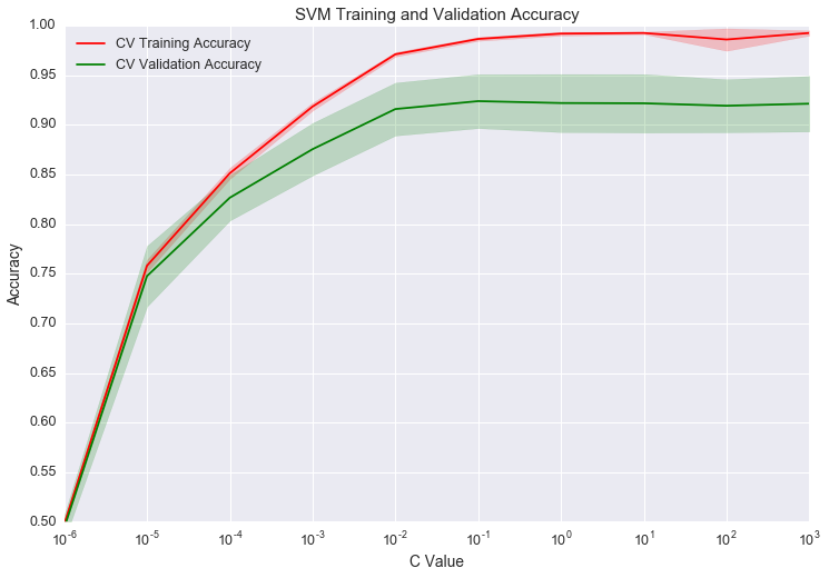
From the graph, it looks like the best value of C is at 10-1. The validation accuracy begins slowly decreasing after that 10-1, indicating we are overfitting. The validation curve looks great, but we only optimized on C. We don’t have to use a linear kernel. We could do a grid search on different kernels and C values. With a larger search space, we might get a different set of optimal parameters.
Let’s run a parameter grid search to see what the optimal parameters are for the SVM model. We’ll switch to the general Support Vector Classifier in sklearn so we can have the option to try non-linear kernels.
from sklearn.svm import SVC

Cs = np.logspace(-6, 3, 10)
parameters = [{'kernel': ['rbf'], 'C': Cs},
              {'kernel': ['linear'], 'C': Cs}]

svc = SVC(random_state = 12)

clf = GridSearchCV(estimator = svc, param_grid = parameters, cv = 5, n_jobs = -1)
clf.fit(x_train.values, y_train.values.flatten())

print clf.best_params_
print clf.best_score_
{'kernel': 'rbf', 'C': 1000.0}
0.925968842539
So the best cross-validated parameters are a rbf kernel with C = 1000. Let’s use the best model to predict on the test data.
clf.score(x_test, y_test)
0.94339025932953824
94% accuracy. That seems pretty high. But how do we know how good that actually is?
Evaluating the Model
How much better is the model than the no-information rate model? The no-information rate is the accuracy we’d get if we guessed the most common class for every observation. It’s the best we could do with no features.
y_test.activity_id.value_counts().values[0] / y_test.activity_id.value_counts().values.sum()
0.17583807716635041
Our model’s accuracy of 94% looks even better compared to the baseline of 18%. That’s over five times more accurate than the no-information accuracy. But where does our model fail? Let’s look at the crosstab.
crosstab = pd.crosstab(y_test.values.flatten(), clf.predict(x_test),
                          rownames=['True'], colnames=['Predicted'],
                          margins=True)
crosstab
| Predicted | 1 | 2 | 3 | 4 | 5 | 6 | 7 | 8 | 9 | 10 | 11 | 12 | All |
|---|---|---|---|---|---|---|---|---|---|---|---|---|---|
| True | |||||||||||||
| 1 | 488 | 4 | 4 | 0 | 0 | 0 | 0 | 0 | 0 | 0 | 0 | 0 | 496 |
| 2 | 20 | 449 | 1 | 0 | 0 | 0 | 1 | 0 | 0 | 0 | 0 | 0 | 471 |
| 3 | 5 | 16 | 399 | 0 | 0 | 0 | 0 | 0 | 0 | 0 | 0 | 0 | 420 |
| 4 | 0 | 2 | 0 | 453 | 52 | 0 | 0 | 1 | 0 | 0 | 0 | 0 | 508 |
| 5 | 0 | 0 | 0 | 19 | 536 | 0 | 1 | 0 | 0 | 0 | 0 | 0 | 556 |
| 6 | 0 | 0 | 0 | 0 | 0 | 544 | 0 | 0 | 0 | 0 | 1 | 0 | 545 |
| 7 | 0 | 1 | 0 | 3 | 0 | 0 | 16 | 1 | 1 | 0 | 1 | 0 | 23 |
| 8 | 0 | 0 | 0 | 0 | 0 | 0 | 0 | 10 | 0 | 0 | 0 | 0 | 10 |
| 9 | 0 | 0 | 0 | 0 | 0 | 0 | 1 | 0 | 20 | 0 | 11 | 0 | 32 |
| 10 | 0 | 0 | 0 | 0 | 0 | 0 | 0 | 0 | 0 | 19 | 0 | 6 | 25 |
| 11 | 0 | 0 | 0 | 1 | 0 | 1 | 1 | 0 | 11 | 1 | 34 | 0 | 49 |
| 12 | 0 | 0 | 0 | 0 | 0 | 0 | 0 | 0 | 0 | 9 | 3 | 15 | 27 |
| All | 513 | 472 | 404 | 476 | 588 | 545 | 20 | 12 | 32 | 29 | 50 | 21 | 3162 |
We do really well for activity_ids 1-3, 5, 6, and 8, but much worse for 4, 7, and 9-12. Why is that?
One possible answer is that we don’t have enough data. The All column on the right side of the crosstab indicates that we have way fewer observations for activities 7-12. Getting more data may improve the model, depending on whether it’s a bias or variance issue.
Additionally, it’s clear the model seems to be systematically mistaking some activities for others (activities 4 and 5, 9 and 11, and 10 and 12 are confused for each other more than others). Maybe there’s a reason for this. Let’s put the labels on the activity_ids and see if we notice any patterns.
crosstab_clean = crosstab.iloc[:-1, :-1]
crosstab_clean.columns = activity_df.activity_label.values
crosstab_clean.index = activity_df.activity_label.values
crosstab_clean
| WALKING | WALKING _UPSTAIRS | WALKING _DOWNSTAIRS | SITTING | STANDING | LAYING | STAND_ TO_SIT | SIT_ TO_STAND | SIT_ TO_LIE | LIE_ TO_SIT | STAND_ TO_LIE | LIE_ TO_STAND | |
|---|---|---|---|---|---|---|---|---|---|---|---|---|
| WALKING | 488 | 4 | 4 | 0 | 0 | 0 | 0 | 0 | 0 | 0 | 0 | 0 |
| WALKING_ UPSTAIRS | 20 | 449 | 1 | 0 | 0 | 0 | 1 | 0 | 0 | 0 | 0 | 0 |
| WALKING_ DOWNSTAIRS | 5 | 16 | 399 | 0 | 0 | 0 | 0 | 0 | 0 | 0 | 0 | 0 |
| SITTING | 0 | 2 | 0 | 453 | 52 | 0 | 0 | 1 | 0 | 0 | 0 | 0 |
| STANDING | 0 | 0 | 0 | 19 | 536 | 0 | 1 | 0 | 0 | 0 | 0 | 0 |
| LAYING | 0 | 0 | 0 | 0 | 0 | 544 | 0 | 0 | 0 | 0 | 1 | 0 |
| STAND_ TO_SIT | 0 | 1 | 0 | 3 | 0 | 0 | 16 | 1 | 1 | 0 | 1 | 0 |
| SIT_ TO_STAND | 0 | 0 | 0 | 0 | 0 | 0 | 0 | 10 | 0 | 0 | 0 | 0 |
| SIT_ TO_LIE | 0 | 0 | 0 | 0 | 0 | 0 | 1 | 0 | 20 | 0 | 11 | 0 |
| LIE_ TO_SIT | 0 | 0 | 0 | 0 | 0 | 0 | 0 | 0 | 0 | 19 | 0 | 6 |
| STAND_ TO_LIE | 0 | 0 | 0 | 1 | 0 | 1 | 1 | 0 | 11 | 1 | 34 | 0 |
| LIE_ TO_STAND | 0 | 0 | 0 | 0 | 0 | 0 | 0 | 0 | 0 | 9 | 3 | 15 |
That makes it way more clear. The model struggles to classify those activity_ids because they are similar actions. 4 and 5 are both stationary (sitting and standing), 9 and 11 both involving lying down (sit_to_lie and stand_to_lie), and 10 and 12 both involve standing up from a resting position (lie_to_sit and lie_to_stand). It makes sense that accelerometer and gyroscope data on these actions would be similar.
So with 94% accuracy in this activity classifier scenario, can we start a $3 Billion dollar fitness tracker company? Maybe.
For the simple Fitbit bracelet, we don’t really need to distinguish between the 12 different activities themselves–only whether or not the person is walking. If we could predict whether someone is walking or not from the smartphone with near perfect accuracy, we’d be in business.
Predicting Walking vs. Not Walking
So how do we classify walking? First we need to convert the labels to a binary to indicate whether they represent walking or staying in place. From the activity labels, we know that 1-3 are walking and everything other activity involves staying in place.
y_train['walking_flag'] = y_train.activity_id.apply(lambda x: 1 if x <= 3 else 0)
y_test['walking_flag'] = y_test.activity_id.apply(lambda x: 1 if x <= 3 else 0)
Now, we’ll train a new SVM model and find the optimal parameters with cross-validation.
from sklearn.svm import SVC

Cs = np.logspace(-6, 3, 10)
parameters = [{'kernel': ['rbf'], 'C': Cs},
              {'kernel': ['linear'], 'C': Cs}]

svc = SVC(random_state = 12)

clf_binary = GridSearchCV(estimator = svc, param_grid = parameters, cv = 5, n_jobs = -1)
clf_binary.fit(x_train.values, y_train.walking_flag.values.flatten())

print clf_binary.best_params_
print clf_binary.best_score_
{'kernel': 'linear', 'C': 0.10000000000000001}
0.999098751127
clf_binary.score(x_test, y_test.walking_flag)
0.99905123339658441
99.9% accuracy! Let’s look at the crosstab.
crosstab_binary = pd.crosstab(y_test.walking_flag.values.flatten(), clf_binary.predict(x_test),
                          rownames=['True'], colnames=['Predicted'],
                          margins=True)
crosstab_binary
| Predicted | 0 | 1 | All |
|---|---|---|---|
| True | |||
| 0 | 1774 | 1 | 1775 |
| 1 | 2 | 1385 | 1387 |
| All | 1776 | 1386 | 3162 |
That’s beautiful! We can almost perfectly tell when someone is walking from smartphone accelerometer and gyroscope data. Now we just need a second model to estimate the distance traveled and we’ll be ready to compete with Fitbit.
For those interested, the Jupyter Notebook with all the code can be found in the Github repository for this post.
Leave a Comment