

Evaluating Models With Small Data
Big data is everywhere. In the past five years, data scientists and software engineers have increasingly turned to technologies like Apache Spark and GPU acceleration to build powerful models and make sense of the data. I don’t see this trend changing any time soon. In fact, I think it should be increasing. That’s why I spend my days helping bring GPU accelerated data science tools to market, so people can easily and efficiently analyze data at scale (check out NVIDIA’s RAPIDS project for more information).
But some important problems simply don’t provide big data. Patient outcomes data from clinical trials, for example, isn’t likely to have more than a couple hundred observations (often far less, actually). More generally, when the cost of generating data is high, the cost of labeling data is high, or the time and effort involved in collecting the data is significant, we often have to deal with small datasets. Building models on these datasets poses a different and subtle set of challenges.
Why Small Datasets Are Different
I’m sure someone could list dozens of reasons modeling on small datasets is different than modeling on large datasets. But, I’m going to focus on the one I’ve seen most frequently overlooked: we can’t rely on the same statistical properties that give us confidence in our standard evaluation metrics.
It’s generally good practice to think of most datasets (large and small) as being drawn from some unknown true data generating process. This means our dataset is already a sample population of the true data universe.
Standard Evaluation Metrics are Point Estimates
We don’t often think about it, but the standard model evaluation metrics of accuracy, precision, and recall are only point estimates. They’re estimates of the true value based on our sample data, and, though we may not think about it, they come with uncertainty. Most importantly, when we split an already small dataset into training, validation, and test datasets, we end up magnifying our risk of biased evaluation metrics.
We have an innate tendency to trust point estimates, and it’s not surprising. Point estimates are easy. Reporting 92% accuracy is easier and sounds better than reporting 92% +- 4%. But this difference isn’t just academic. The difference between an accuracy of 88% and 96% could literally be the difference between a company launching and shelving a product.
Measuring Metric Uncertainty
One of the easiest ways to measure the uncertainty of your metrics is to simply repeatedly sample and fit multiple models. This won’t account for any sampling differences in our data compared to the true “universe”, but it will help us minimize the risk of simply getting a “lucky split” when we split our training and validation data. Below, I’ll walk through some example code of how to do this:
First, I’ll import a few libraries and load an example dataset from scikit-learn.
import numpy as np
import pandas as pd
from sklearn.datasets import load_breast_cancer
from sklearn.ensemble import RandomForestClassifier
from sklearn.model_selection import train_test_split
from sklearn import metrics
import matplotlib.pyplot as plt
%matplotlib inline
data = load_breast_cancer()
features, target = data.data, data.target
features.shape, target.shape
((569, 30), (569,))
There are 569 records in the data and 30 features. To drive the point of this post home, I’ll further sample to only 50 observations and pick three features at random.
np.random.seed(12)

cols = np.random.choice(features.shape[1], 3)
features = features[:, cols]

sample_indices = np.random.choice(np.arange(0, len(features)), 50)
features, target = features[sample_indices, :], target[sample_indices]
With the data defined, I can create few functions to prepare my data, fit a model, and predict on a dataset. These are just wrappers around scikit-learn functionality for convenience. First, I’ll define a function to randomly partition my data into training and validation sets.
def partition_data(features, labels, test_size, seed):
    x_train, x_test, y_train, y_test = train_test_split(
        features, labels, test_size=test_size, random_state=seed)
    return x_train, x_test, y_train, y_test
Next, I’ll define a function to take an instantiated model and fit it to some training data.
def fit_model(model, features, labels):
    model.fit(features, labels)
Finally, I’ll define a function to use the fit model to make predictions. I’ll make sure to use the predict_proba method because I want to vary the threshold at which I consider a prediction belonging to one class or the other.
def predict(model, features):
    return model.predict_proba(features)
Next, I need a function to compute my evaluation metrics. Because I care more about some types of errors than the others, I’m interested in measuring precision and recall. I’ll define a function to take my validation labels and predictions and compute precision and recall at various “decision thresholds”. When the decision threshold is 0.5, any prediction of 0.5 or above will be considered a positive class. If the threshold were raised to be 0.8, only predictions above 0.8 would be considered the positive class. By varying the threshold and computing our metrics, we can generate what’s typically called a precision recall curve.
There’s a scikit-learn function to generate the precision-recall curve data, but it doesn’t use consistent thresholds across different samples of small datasets, for the very reasons discussed above!
def calculate_precision_recall_at_thresholds(y_true, y_preds, stepsize=0.01):
    tuplesList = []

    # Need to limit the maximum threshold to avoid having no positive predictions
    limit = np.floor(max(y_preds))

    for i in np.arange(0, limit, stepsize):
        thresholdedLabels = list(map(lambda x: 1 if x >= i else 0, y_preds))
        precision = metrics.precision_score(y_true, thresholdedLabels)
        recall = metrics.recall_score(y_true, thresholdedLabels)
        tuplesList.append( (precision, recall, i) )

    precision = [x[0] for x in tuplesList]
    recall = [x[1] for x in tuplesList]
    thresholds = [x[2] for x in tuplesList]

    return precision, recall, thresholds
There are some statistical concerns with this function, and first among them is the fact that I’m simply ignoring situations in which a decision threshold of 0.97 (for example) would result in no positive class predictions. This matters, but since we’re trying to be quick and dirty it’s fine as it is.
With these functions defined, I’m ready to run my experiment. I’ll wrap these into a single main function and collect the precision and recall data for every iteration.
def main(features, labels, N=5, test_size=0.33, stepsize=0.01, seed=None):
    results = pd.DataFrame(columns=['precision', 'recall', 'threshold', 'iteration_seed'])

    for i in range(N):
        if not seed:
            current_seed = np.random.randint(1000000)

        if i % 10 == 0:
            print(i, current_seed)

        x_train, x_test, y_train, y_test = partition_data(features, labels, test_size, current_seed)

        clf_rf = RandomForestClassifier(n_estimators=100, verbose=False, random_state=current_seed , n_jobs=-1)
        fit_model(clf_rf, x_train, y_train)
        test_preds = predict(clf_rf, x_test)

        precision, recall, thresholds = calculate_precision_recall_at_thresholds(y_test, test_preds[:, 1], stepsize=stepsize)

        partial_results = pd.DataFrame({'precision':precision,
                           'recall':recall,
                           'threshold':thresholds,
                           'iteration_seed':float(current_seed)})

        results = results.append(partial_results)

    return results
All set. Time to run the experiment! I’m printing the iteration number every 10 iterations because I like to see my progress.
N = 20
stepsize = 0.01
test_size = 0.33
seed = None

out = main(features, target, N, test_size, stepsize, seed=None)
0 61795
10 952425
With the data in hand, I can calculate the standard deviation at each decision threshold from the runs of my experiment. Then, I can plot the results.
results = out.groupby(['threshold'], as_index=False).agg(
    {'precision': ['mean', 'std', 'min', 'max'],
     'recall': ['mean', 'std', 'min', 'max']})

meanRecall = results['recall']['mean']
meanPrecision = results['precision']['mean']
stdPrecision = results['precision']['std']

fig, ax = plt.subplots(figsize=(10, 10))
plt.title(
    'Average Precision-Recall Curve with Std. Deviation\nCalculated from {0} Random Partitions'.format(N)
    , fontsize='14')

ax.set_xlabel('Recall')
ax.set_ylabel('Precision')
ax.set_ylim([0.0, 1.01])
ax.set_xlim([0.0, 1.01])
ax.set_yticks(np.arange(0, 1.01, .05))

ax.plot(meanRecall, meanPrecision, label='Mean Precision-Recall Curve', alpha = 1.0, color='black')
ax.fill_between(meanRecall, meanPrecision-stdPrecision, meanPrecision+stdPrecision,
    alpha=0.5, facecolor='blue')


for i, (x, y, label) in enumerate(zip(meanRecall, meanPrecision, results['threshold'])):
    if i % 5 == 0:
        ax.annotate(
            np.round(label,2),
            color='black',
            xy=(x, y),
            textcoords='data'
        )

ax.legend(loc="lower left")
plt.grid()
plt.show()
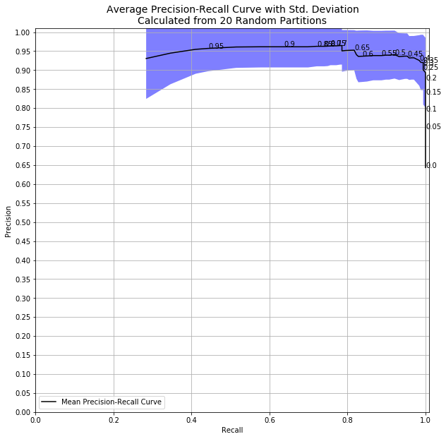
Right away, it’s clear that there is huge uncertainty in my metrics at high decision thresholds! The randomness in my splitting into train and test datasets, combined with the randomness in my model, resulted in a huge variation in my precision and recall metrics. We can see this in results data itself, too.
results[results.threshold > .95]
| threshold | precision | recall | |||||||
|---|---|---|---|---|---|---|---|---|---|
| mean | std | min | max | mean | std | min | max | ||
| 95 | 0.95 | 0.957283 | 0.060039 | 0.857143 | 1.0 | 0.442526 | 0.229691 | 0.100000 | 0.800000 |
| 96 | 0.96 | 0.957283 | 0.060039 | 0.857143 | 1.0 | 0.442526 | 0.229691 | 0.100000 | 0.800000 |
| 97 | 0.97 | 0.954832 | 0.064307 | 0.833333 | 1.0 | 0.410431 | 0.233079 | 0.100000 | 0.800000 |
| 98 | 0.98 | 0.944795 | 0.081874 | 0.750000 | 1.0 | 0.345867 | 0.206159 | 0.076923 | 0.727273 |
| 99 | 0.99 | 0.930672 | 0.106333 | 0.666667 | 1.0 | 0.283582 | 0.178153 | 0.076923 | 0.666667 |
With a decision threshold of 0.98, we had precision as low as 0.75 and as high as 1.0! If the decision to take a model to production is made based on hitting specified levels of precision and recall, you might be changing your product or service based on pure luck of the draw. As crazy as it sounds, things like this happen all the time.
Does This Matter?
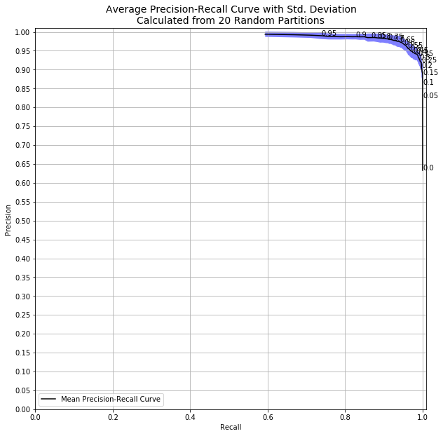
So how much does this matter? If I had run the same code with all 569 observations instead of only 50, we’d see this:
results[results.threshold > .95]
| threshold | precision | recall | |||||||
|---|---|---|---|---|---|---|---|---|---|
| mean | std | min | max | mean | std | min | max | ||
| 95 | 0.95 | 0.990041 | 0.008778 | 0.975309 | 1.0 | 0.738581 | 0.035483 | 0.655462 | 0.788136 |
| 96 | 0.96 | 0.990041 | 0.008778 | 0.975309 | 1.0 | 0.738581 | 0.035483 | 0.655462 | 0.788136 |
| 97 | 0.97 | 0.991422 | 0.007243 | 0.977528 | 1.0 | 0.711212 | 0.033583 | 0.638655 | 0.769841 |
| 98 | 0.98 | 0.992716 | 0.007226 | 0.976471 | 1.0 | 0.666782 | 0.048689 | 0.549180 | 0.746032 |
| 99 | 0.99 | 0.993946 | 0.006915 | 0.984375 | 1.0 | 0.593369 | 0.065964 | 0.467213 | 0.682927 |
With a decision threshold of 0.98, we had standard deviation of 0.7% and precision of at least 97.5% every single time. Going from 50 to 500 samples dramatically affects the both the quality and certainty of my model.
Conclusion
While big data and its challenges dominate the news, small data comes with challenges of its own. Measuring the uncertainty of our model evaluation metrics is crucially important when modeling on small data, because we can’t rely on the central limit theorem. In the code above, we walked through a quick and easy way to be more informed about the quality of our models.
When you care about one class more than the other, you’re often willing to tolerate some small degree of false positives if it dramatically improves your ability to correctly identify more of your class of interest. Google Photos might prefer their location recognition service have a false positive rate of 2% with a recall of 97% than a false positive rate of 1% with a recall of 85%. Measuring the uncertainty of your metrics is a great to way be confident in your assessment.
Leave a Comment