Deep learning is all the rage right now. Convolutional neural networks are particularly hot, achieving state of the art performance on image recognition, text classification, and even drug discovery.

Since I didn’t take any courses on deep learning in college, I figured I should start at the core of convolutional nets to really understand them. In a series of posts, I’ll walk through convolution, standard neural networks, and convolutional networks in Python/Tensorflow.

So here we go. Time to dive into image transformation with convolution.

What is Convolution?

In math, convolution is essentially the blending of two functions into a third function. In the context of image processing, convolution is kind of like transforming image pixels in a structured way, taking nearby pixels into account. In terms of coding, let’s think of an image as a 2-D array of pixels with 3 channels (reg, green, and blue). I’m going to abstract away from the color aspect of the image (so grayscale only), but the logic of this post extends naturally to the multichannel 2-D image. We want to transform each element of the array in a structured way, taking into account nearby elements.

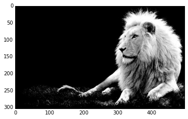
Let’s look at an image and its pixel array. For this post, I’ll download a grayscale picture of a lion from Google Images. The lion image I’m using comes from here.

import numpy as np
from PIL import Image
from scipy import misc
from skimage import data
from skimage.color import rgb2gray
import matplotlib.pyplot as plt
%matplotlib inline
import requests
from StringIO import StringIO
from __future__ import division

response = requests.get('http://vignette2.wikia.nocookie.net/grayscale/images/4/47/Lion.png/revision/latest?cb=20130926182831')
lion_arr = np.array(Image.open(StringIO(response.content)))

First let’s see the lion.

plt.imshow(lion_arr)

Looks good. However, though it does look grayscale, this image actually still has three channels (red, green, and blue). We can see that by looking at the shape of the array. Maybe all the color channels are actually the same?

print lion_arr.shape
print np.array_equal(lion_arr[:, :, 0], lion_arr[:, :, 1])
print np.array_equal(lion_arr[:, :, 1], lion_arr[:, :, 2])

(303, 497, 3)
True
True

Perfect. If we imagine this 3-D array as 3 separate 2-D arrays, each 2-D array is identical. Let’s just use the first channel as the image.

lion_arr = lion_arr[:, :, 0]

Let’s take a look at the image array. We’ve got rows and columns of numbers between 0 and 255 representing pixels.

lion_arr[:200, :400]

array([[  0,   0,   0, ...,   0,   0,   0],
       [  2,   2,   1, ...,   0,   0,   0],
       [  0,   0,   0, ...,   0,   0,   0],
       ..., 
       [  0,   1,   0, ...,   5,  86,  97],
       [  0,   1,   0, ...,  56, 114, 114],
       [  0,   1,   0, ..., 122, 130, 143]], dtype=uint8)

If we wanted to perform a convolution on the array, we’d loop through and transform each element in the same way. We’ll define a 2-D kernel that we’ll then apply to (multiply with) every element in the array. But how do we actually use the 2-D kernel?

Convolution with 2-D Kernels

With a 2-D kernel, we need to apply our kernel to patches of the image with the same shape as the kernel. Since we still want to output a scalar from our convolution, we’ll multiply our kernel and the patch and then take the sum of the resulting output array.

There’s a problem though. Imagine sequentially moving a 3 x 3 patch through a 5 x 5 image. You’d start with the top left corner, and move across the image until you hit the top right corner. That would only take take 3 moves. By this logic, we’d end up with a smaller image than we started with. To avoid this, we pad the array with zeros on every side. The zeros allow us to apply our kernel to every pixel.

More generally, to pass an m x m kernel over a p x q image, we’d need to pad the image with m - 2 zeros on every side (where m is an odd number). We assume m is odd so that the kernel has a “center”.

Time to do it. I’ll convolve a 3 x 3 kernel on the lion image. First I’ll pad the array with a zero at the end of each row and column. Then I’ll define a 3 x 3 kernel, pass it over every 3 x 3 patch in the padded image, and do elementwise multiplication of the 3 x 3 kernel and 3 x 3 array. I’ll store the sum of that transformation in an output array, which will be the same size as our original lion array.

padded_array = np.pad(lion_arr, (1, 1), 'constant')
kernel = np.array([[0, 0, 0], [0, 1, 0], [0, 0, 0]])
output_array = np.zeros(lion_arr.shape)

for i in xrange(padded_array.shape[0]-2):
    for j in xrange(padded_array.shape[1]-2):
        temp_array = padded_array[i:i+3, j:j+3]
        output_array[i, j] = np.sum(temp_array*kernel)

Let’s look at the output.

plt.imshow(output_array, cmap = plt.get_cmap('gray'))

It’s the same! Why? Because of the kernel we chose. For any given patch in the image, our convolution is just outputting 1 * the middle element of the patch. Every other element-to-element multiplication becomes 0 due to the kernel. For this reason, we call this kernel the identity kernel.

Standard Convolution

Let’s go through the example kernels listed on this wikipedia page. First, I’ll define a function to convolve a 2-D kernel on an image. Since we’re calculating sums, our output values can be greater than 255 or less than 0. We might want to squash those values to 255 and 0, respectively, so I’ll write a function to do that. There are better ways to handle this phenomenon (such as biasing the output value by a certain amount), but this works for now.

def squash_pixel_value(value):
    if value < 0:
        return 0
    elif value < 255:
        return value
    else:
        return 255

def conv_2d_kernel(image_array_2d, kernel, squash_pixels = True):
    padded_array = np.pad(image_array_2d, (1, 1), 'constant')
    
    kernel_width = kernel.shape[0]
    kernel_height = kernel.shape[1]
    
    transformed_array = np.zeros(image_array_2d.shape)
 
    for i in xrange(padded_array.shape[0] - kernel_width + 1):
        for j in xrange(padded_array.shape[1] - kernel_height + 1):
            temp_array = padded_array[i:i+kernel_width, j:j+kernel_height]
            #print temp_array.shape
            if squash_pixels:
                transformed_array[i, j] = squash_pixel_value(np.sum(temp_array*kernel))
            else:
                transformed_array[i, j] = np.sum(temp_array*kernel)
    return transformed_array

All set. We’re ready to go through each transformation on the wikipedia page. Let’s see how they turn out.

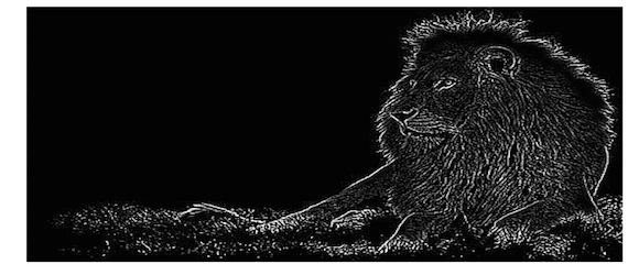
Edge Detection

edge_kernel_1 = np.array([[1, 0, -1],
                          [0, 0, 0],
                          [-1, 0, 1]])

edge_kernel_2 = np.array([[0, 1, 0],
                          [1, -4, 1],
                          [0, 1, 0]])

edge_kernel_3 = np.array([[-1, -1, -1],
                          [-1, 8, -1],
                          [-1, -1, -1]])

lion_transf_edge1 = conv_2d_kernel(lion_arr, kernel = edge_kernel_1, squash_pixels = True)
lion_transf_edge2 = conv_2d_kernel(lion_arr, kernel = edge_kernel_2, squash_pixels = True)
lion_transf_edge3 = conv_2d_kernel(lion_arr, kernel = edge_kernel_3, squash_pixels = True)

f, ax_array = plt.subplots(2, 2)
f.set_figheight(10)
f.set_figwidth(15)
ax_array[0, 0].imshow(lion_arr, cmap = plt.get_cmap('gray'))
ax_array[0, 0].set_title('Original Image')
ax_array[0, 0].axis('off')
ax_array[0, 1].imshow(lion_transf_edge1, cmap = plt.get_cmap('gray'))
ax_array[0, 1].set_title('Edge Kernel 1')
ax_array[0, 1].axis('off')
ax_array[1, 0].imshow(lion_transf_edge2, cmap = plt.get_cmap('gray'))
ax_array[1, 0].set_title('Edge Kernel 2')
ax_array[1, 0].axis('off')
ax_array[1, 1].imshow(lion_transf_edge3, cmap = plt.get_cmap('gray'))
ax_array[1, 1].set_title('Edge Kernel 3')
ax_array[1, 1].axis('off')

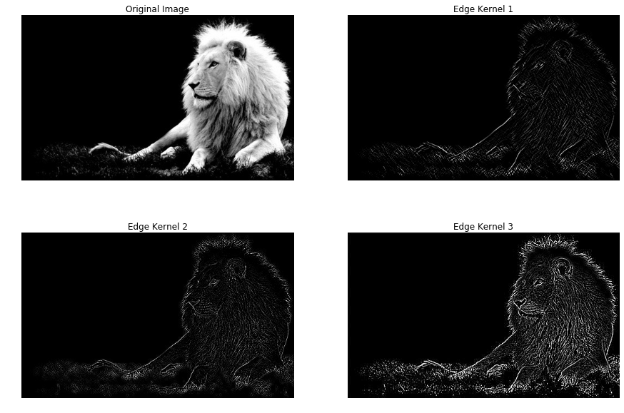
Awesome! Looks like each of the edge kernels make the edges successively more distinct.

Sharpen

sharpen_kernel = np.array([[0, -1, 0],
                           [-1, 5, -1],
                           [0, -1, 0]])

unsharp_kernel = np.array([[1, 4, 6, 4, 1],
                           [4, 16, 24, 16, 4],
                           [6, 24, -476, 24, 6],
                           [4, 16, 24, 16, 4],
                           [1, 4, 6, 4, 1]]) / -256

lion_transf_sharpen = conv_2d_kernel(lion_arr, kernel = sharpen_kernel, squash_pixels = True)
lion_transf_unsharp = conv_2d_kernel(lion_arr, kernel = unsharp_kernel, squash_pixels = True)

f, ax_array = plt.subplots(3, 1)
f.set_figheight(15)
f.set_figwidth(12)
ax_array[0].imshow(lion_arr, cmap = plt.get_cmap('gray'))
ax_array[0].set_title('Original Image')
ax_array[0].axis('off')
ax_array[1].imshow(lion_transf_sharpen, cmap = plt.get_cmap('gray'))
ax_array[1].set_title('Sharpen Kernel')
ax_array[1].axis('off')
ax_array[2].imshow(lion_transf_unsharp, cmap = plt.get_cmap('gray'))
ax_array[2].set_title('Unsharp Kernel')
ax_array[2].axis('off')

(-0.5, 496.5, 302.5, -0.5)

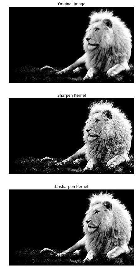
These look good, too. The convolution with the sharpen kernel clearly sharpened the image, and the unsharp kernel does look slightly sharper than the original image (though not by much).

Blur

blur_box_kernel = np.ones((3, 3)) / 9
blur_gaussian_kernel = np.array([[1,2,1],
                                 [2,4,2],
                                 [1,2,1]]) / 16

lion_transf_blur_box = conv_2d_kernel(lion_arr, kernel = blur_box_kernel, squash_pixels = True)
lion_transf_blur_gaussian = conv_2d_kernel(lion_arr, kernel = blur_gaussian_kernel, squash_pixels = True)

f, ax_array = plt.subplots(3, 1)
f.set_figheight(15)
f.set_figwidth(12)

ax_array[0].imshow(lion_arr, cmap = plt.get_cmap('gray'))
ax_array[0].set_title('Original Image')
ax_array[0].axis('off')
ax_array[1].imshow(lion_transf_blur_box, cmap = plt.get_cmap('gray'))
ax_array[1].set_title('Box Kernel Blur')
ax_array[1].axis('off')
ax_array[2].imshow(lion_transf_blur_gaussian, cmap = plt.get_cmap('gray'))
ax_array[2].set_title('Gaussian Kernel Blur')
ax_array[2].axis('off')

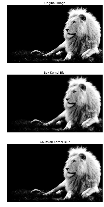
Definitely blurrier.

Okay. So I’ve got the convolution math and application down. Since I’m going to eventually build a convolutional neural net using Tensorflow, I should really understand Tensorflow’s 2-D convolution function, nn.conv2d. So how does it work?

Convolution in Tensorflow

From the documentation, conv2d:

Computes a 2-D convolution given 4-D input and filter tensors. Given an input tensor of shape [batch, in_height, in_width, in_channels] and a filter / kernel tensor of shape [filter_height, filter_width, in_channels, out_channels]

For the input tensor, since we’re only convolving one image, our batch = 1. The in_height and in_width are the dimensions of the image, (303, 497), and in_channels = 1 since we have a grayscale image.

For the kernel tensor, the filter_height and filter_width are the dimensions of the kernel (3, 3). in_channels = 1 since it has to match the input tensor, and out_channels = 1 since we want another grayscale image. So I need to reshape my 2-D arrays into this 4-D shape. I’ll choose the blur kernel for this example.

lion_array_4d = lion_arr.reshape(-1, 303, 497, 1)
blur_kernel_4d = blur_box_kernel.reshape(3, 3, 1, 1)

Understanding the next code block requires some knowledge of Tensorflow, so if anyone is interested in learning about it I recommend checking out one of Google’s tutorials.

import tensorflow as tf

graph = tf.Graph()
with graph.as_default():
    tf_input_image = tf.Variable(np.array(lion_array_4d, dtype = np.float32))
    tf_blur_kernel = tf.Variable(np.array(blur_kernel_4d, dtype = np.float32))    
    tf_convolution_output = tf.nn.conv2d(tf_input_image, tf_blur_kernel, strides = [1, 1, 1, 1], padding = 'SAME')

with tf.Session(graph = graph) as sess:
    tf.initialize_all_variables().run()
    transformed_image = tf_convolution_output.eval()
    transformed_image = transformed_image[0, :, :, 0]

So what did that code do? In the first with statement, I initialized the input and kernel tensors (with values as floats) and the convolution. In the second with statement, I executed the tensorflow graph and evaluated the convolution. Conv2d also needs parameters strides and padding. strides = [1, 1, 1, 1] results in a convolution on every pixel and padding = 'SAME' is the standard zero padding that results in an output array with the same shape as the input array.

Our new output array should be the same as our hand-calculated output array lion_transf_blur_box. I’ll test whether they are equal to 4 decimal places using np.testing.assert_array_almost_equal. If they aren’t equal, this will throw an error.

np.testing.assert_array_almost_equal(lion_transf_blur_box, transformed_image,
                             decimal = 4)

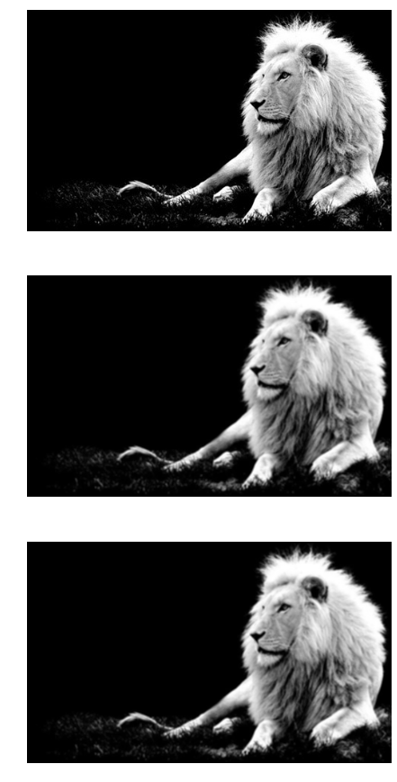
Perfect! I got the same output using my conv_2d_kernel function and tensorflow’s tf.nn.conv2d function. Let’s compare the original image, the original blur, and the new blur.

f, ax_array = plt.subplots(3, 1)
f.set_figheight(15)
f.set_figwidth(12)
ax_array[0].imshow(lion_arr, cmap = plt.get_cmap('gray'))
ax_array[0].axis('off')
ax_array[1].imshow(lion_transf_blur_box, cmap = plt.get_cmap('gray'))
ax_array[1].axis('off')
ax_array[2].imshow(transformed_image, cmap = plt.get_cmap('gray'))
ax_array[2].axis('off')

Next Steps

I’ve got a pretty good handle on convolution for image analysis at this point. But it’s not clear how we go from this to convolutional neural networks. In the next post, I’ll walk through a simple neural network, and then eventually build a convolutional net.